Calculus Honors · AP-aligned study guide

6.2 · Separation of variables, growth, and logistic models

Solve separable initial-value problems, preserve equilibrium solutions, and interpret exponential or logistic behavior.

AP 7.6–7.8; logistic: BC 7.9 · Reading: Larson & Edwards §§6.2–6.3

Learning objectives

  • Separate and solve a differential equation with initial data.
  • Identify equilibrium solutions before dividing by a dependent variable.
  • Interpret growth parameters and carrying capacity.

Separate variable factors and integrate

For dydx=g(x)h(y)\displaystyle \frac{dy}{dx}=g(x)h(y), put dy/h(y)\displaystyle dy/h(y) on one side and g(x)dx\displaystyle g(x)dx on the other, then integrate. Check solutions with h(y)=0\displaystyle h(y)=0 before dividing; these equilibrium solutions may otherwise be lost.

For y′=2xy\displaystyle y'=2xy, the nonzero solutions satisfy dy/y=2x dx\displaystyle dy/y=2x\,dx. Integration gives ln⁡∣y∣=x2+C\displaystyle \ln|y|=x^2+C, or y=Cex2\displaystyle y=Ce^{x^2}. The family also includes y=0\displaystyle y=0 when the multiplicative constant is zero.

Exponential growth is proportional to amount

The model P′=kP\displaystyle P'=kP has solution P(t)=P0ekt\displaystyle P(t)=P_0e^{kt}. Positive k\displaystyle k gives growth and negative k\displaystyle k gives decay. The constant k\displaystyle k has inverse-time units, and the initial amount fixes the coefficient.

If an amount doubles in time T\displaystyle T, then k=ln⁡2/T\displaystyle k=\ln2/T. For a half-life T\displaystyle T, k=−ln⁡2/T\displaystyle k=-\ln2/T. Use logarithms to solve for time; a constant percentage rate is not the same as constant additive growth.

P(t)=P0ektP(t)=P_0e^{kt}

Logistic growth has a limiting capacity

The BC logistic model P′=kP(1−P/K)\displaystyle P'=kP(1-P/K) has equilibria 0\displaystyle 0 and K\displaystyle K, with positive constants k\displaystyle k and K\displaystyle K. For 0<P<K\displaystyle 0<P<K, the amount grows toward carrying capacity K\displaystyle K. Above K\displaystyle K, the rate is negative.

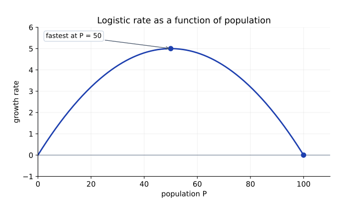
The growth rate is largest at P=K/2\displaystyle P=K/2, because the quadratic rate as a function of P\displaystyle P has its maximum there. The logistic solution is P(t)=K/(1+Ae−kt)\displaystyle P(t)=K/(1+Ae^{-kt}), with A\displaystyle A determined by the initial condition.

Worked examples

A separable initial-value problem

Solve y′=2xy\displaystyle y'=2xy with y(0)=3\displaystyle y(0)=3.

  1. Separate to dy/y=2x dx\displaystyle dy/y=2x\,dx.
  2. Integrate and exponentiate to get y=Cex2\displaystyle y=Ce^{x^2}.
  3. The initial condition gives C=3\displaystyle C=3, so y=3ex2\displaystyle y=3e^{x^2}.

A doubling model

An amount starts at 5\displaystyle 5 and doubles in 3\displaystyle 3 hours. Find its exponential model.

  1. The doubling condition gives e3k=2\displaystyle e^{3k}=2.
  2. Thus k=ln⁡2/3\displaystyle k=\ln2/3.
  3. The model is P(t)=5e(ln⁡2)t/3=5⋅2t/3\displaystyle P(t)=5e^{(\ln2)t/3}=5\cdot2^{t/3}.

Common mistakes

  • Losing equilibrium solutions when dividing by y.
  • Using the initial amount as the exponential rate constant.
  • Confusing fastest logistic growth with carrying capacity.

Try it yourself

No calculator required.

1. Solve y′=3x2y\displaystyle y'=3x^2y with y(0)=2\displaystyle y(0)=2.

Show worked solution

Integrate dy/y=3x2dx\displaystyle dy/y=3x^2dx to get ln⁡∣y∣=x3+C\displaystyle \ln|y|=x^3+C. The initial-value solution is y=2ex3\displaystyle y=2e^{x^3}. The equilibrium y=0\displaystyle y=0 exists but does not satisfy this initial value.

2. An amount starts at 80\displaystyle 80 and has half-life 4\displaystyle 4 years. Find its amount at 8\displaystyle 8 years.

Show worked solution

The model is 80e−(ln⁡2)t/4\displaystyle 80e^{-(\ln2)t/4}. At 8\displaystyle 8 years, two half-lives have elapsed, giving 20\displaystyle 20.

BC extension

3. For P′=0.2P(1−P/100)\displaystyle P'=0.2P(1-P/100), identify equilibria, carrying capacity, and the amount at fastest growth.
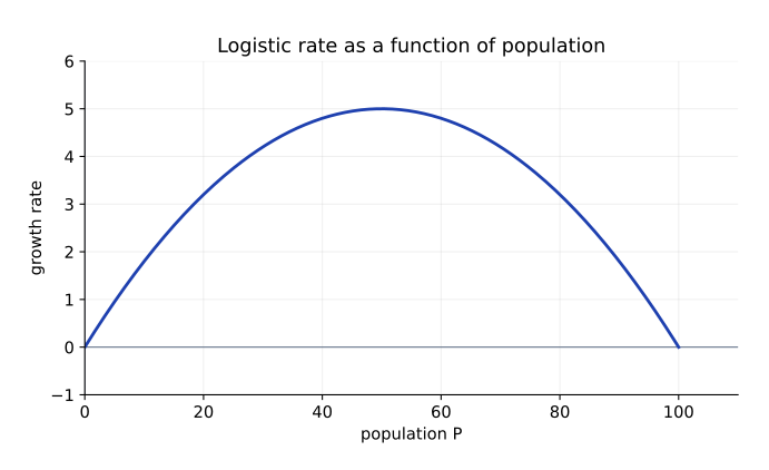
The rate 0.2P times (1 minus P over 100) is a downward parabola with zeros at 0 and 100.
The horizontal axis is population, not time.
Show worked solution

Equilibria are P=0\displaystyle P=0 and P=100\displaystyle P=100. Carrying capacity is 100\displaystyle 100. The rate is maximal at P=50\displaystyle P=50. Below capacity the positive population grows toward 100\displaystyle 100; above it, the population decreases.

The rate 0.2P times (1 minus P over 100) is a downward parabola with zeros at 0 and 100. The rate peaks at population 50; the carrying capacity is the equilibrium population 100.
The rate peaks at population 50; the carrying capacity is the equilibrium population 100.

Need help with this topic?

Work through questions with a tutor and get help with the steps you find difficult.

Get help with this topic