
Repair a removable discontinuity
Let for and . Find for continuity.
- For , factor and cancel to obtain .
- The two-sided limit is .
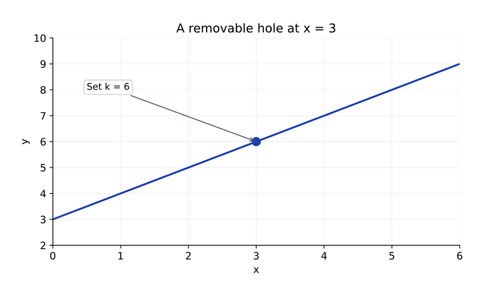
- Continuity requires .
- Choose . The two one-sided limits and the point value now agree.
Calculus Honors · AP-aligned study guide
Test continuity at a point and on an interval, repair removable holes, and use the Intermediate Value Theorem to justify existence claims.
AP topics 1.10–1.13 and 1.16 · Reading: Larson & Edwards §1.4
A function is continuous at x = c if f(c) is defined, the finite two-sided limit exists, and that limit equals f(c). Check the conditions in that order. A graph with a hole can fail the first condition; a jump fails the second; a misplaced filled dot fails the third.
Polynomials are continuous on the real line. Rational functions are continuous wherever their denominator is nonzero. Radicals, logarithms, and trigonometric functions require attention to their domains. Sums, products, and compositions of continuous functions remain continuous wherever the operations are defined.
A removable discontinuity occurs when a finite two-sided limit exists but the function is undefined there or has the wrong value. Setting f(c) equal to that limit repairs the break. A jump has finite but unequal one-sided limits. An infinite discontinuity involves unbounded behavior near the point.
Changing a single point value cannot fix a jump or a vertical asymptote. For , the hole at 1 is removable because the limit is 2. By contrast, a function with left limit 2 and right limit 5 has a jump, regardless of its value at the joining point.
At a joining input c, use the left branch to find the left-hand limit, the right branch to find the right-hand limit, and the branch that includes equality to find f(c). Choose any parameters so all three values agree.
For when x < 2 and when x ≥ 2, the right limit and f(2) are 3. The left limit is . Setting gives a = 1, making the function continuous at the join.
A function is continuous on an open interval if it is continuous at every point inside it. For continuity on [a, b], also require and . At endpoints you approach from inside the interval.
For example, is continuous on [−1, 3]: it is continuous in the interior, right-continuous at −1, and left-continuous at 3. For , the maximal open intervals of continuity are (−∞, 2) and (2, ∞). A denominator restriction cannot be ignored just because the requested interval crosses it.
If f is continuous on [a, b] and N lies strictly between f(a) and f(b), then some c in (a, b) satisfies f(c) = N. The function cannot move continuously between two heights without taking every intermediate height.
For a root, use N = 0 and show opposite signs at the endpoints. State continuity on the whole closed interval, evaluate the endpoints, show that 0 lies between those values, and conclude that at least one root exists in the open interval. IVT does not give an exact root or establish uniqueness.
Opposite signs alone are not enough: has values −1 and 1 at −1 and 1, but it is not continuous on [−1, 1] and never equals 0. The continuity hypothesis prevents this false inference.
If endpoint values have the same sign, IVT gives no root guarantee from those endpoints; a root may still exist. For instance, x² on [−1, 1] has positive endpoint values but has a zero at 0. Distinguish “not guaranteed by these data” from “impossible.”
Let for and . Find for continuity.
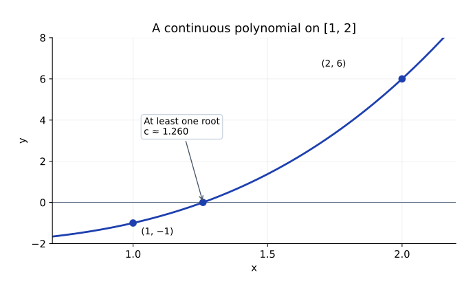
Use IVT to show that has a solution between and .
No calculator required.
1. Let for , and . Find for continuity. Classify the break if .
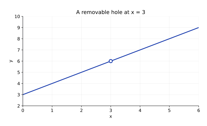
For , cancellation gives . Hence . Continuity requires , so choose . If , the finite limit differs from the point value, so the discontinuity is removable.
2. Let for , and for . Find so that is continuous at .
The left-hand limit is . The right-hand limit and are both . Set , giving . The two one-sided limits and the point value then agree.
3. Use the Intermediate Value Theorem to justify a root of between and . Does IVT alone prove uniqueness?
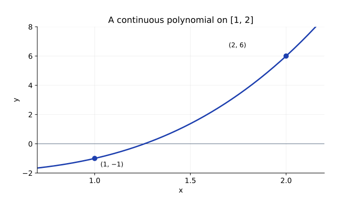
The polynomial is continuous on . Since and , we have . IVT guarantees at least one with . IVT alone does not establish uniqueness.
4. Explain why is continuous on . Then explain why IVT cannot be applied to on .
The square-root function is continuous in the interior, and its endpoint limits agree with its values: and . In contrast, is undefined at , so it is not continuous on . The IVT hypothesis fails.
Work through questions with a tutor and get help with the steps you find difficult.
Get help with this topic